To inspect and run the Portfolio QAOA optimization dataflow on the live canvas, start the Quanifi NiFi container:

docker compose up -d

Verify health status with docker compose ps. Then open https://localhost:8443/nifi in your browser (Username: admin, Password: quanifipassword). The corresponding template JSON is available in demo/qaoa/lanes/qrisp-qaoa.json. For all runtime options, see the Docker Quickstart Guide.

Module 5: Variational Optimization & The Constrained XY Mixer (QAOA)

Move beyond 1990s toy textbook circuits into modern hybrid quantum-classical algorithms. Learn how to solve NP-hard combinatorial business problems using QAOA, and discover how Quanifi enforces hard budget constraints using particle-preserving XY mixers.

1. Beyond Textbook Circuits: The Modern NISQ Era

Algorithms like Deutsch-Jozsa and Grover are brilliant theoretical proofs of quantum speedup, but they require fault-tolerant quantum computers with thousands of noise-free operations.

Today's quantum computers are in the NISQ (Noisy Intermediate-Scale Quantum) era. To extract practical value from noisy hardware, modern quantum software engineering relies on Hybrid Quantum-Classical Algorithms:

💡 The Analogy: GPU Acceleration & Gradient Descent

In machine learning, your CPU runs Python control logic while offloading matrix multiplications to a GPU. Similarly, in a hybrid quantum algorithm:
• The Quantum Processor (QPU) acts as an accelerator that evaluates an objective function in high-dimensional superposition.
• A Classical Optimizer (CPU) iteratively tunes parameterized rotation angles ($\gamma, \beta$) via gradient-free methods (like COBYLA or SPSA) until the minimum energy is found.

2. The Real-World Problem: Markowitz Portfolio Rebalancing

Consider an investment fund managing $n$ candidate assets (e.g. Apple, Google, Microsoft). Each asset $i$ has an expected financial return $\mu_i$, and the mutual volatility between assets is captured by an $n \times n$ covariance matrix $\Sigma$.

The fund manager wants to pick a subset of assets $x \in \{0, 1\}^n$ that maximizes returns while minimizing financial risk, subject to a strict budget constraint: you must select exactly $K$ assets.

The Mathematical Formulation:

$$\min_{x \in \{0,1\}^n} \left( \lambda \sum_{i,j} \Sigma_{ij} x_i x_j - \sum_i \mu_i x_i + P \left( \sum_{i=1}^n x_i - K \right)^2 \right)$$

Where:

$\mu$: Vector of expected returns (we want high returns, hence negative sign).
$\Sigma$: Covariance matrix measuring risk/volatility (we penalize high covariance).
$\lambda \ge 0$: The Risk Factor (how risk-averse the investor is).
$K$: The exact Budget (number of assets to purchase, e.g. $K=2$ out of $3$).
$P > 0$: The penalty weight enforcing the constraint $\sum x_i = K$.

3. How Quantum Solves It: Cost Hamiltonians & The Pauli Mapping

Quantum computers do not understand financial matrices directly. To evaluate this problem on qubits, Quanifi maps classical binary variables $x_i \in \{0, 1\}$ to quantum spin operators (Pauli-$Z$ matrices):

$$x_i = \frac{I - Z_i}{2}$$

When qubit $i$ is in state $\vert 0\rangle$, $Z_i = +1$, so $x_i = \frac{1 - 1}{2} = 0$ (asset not selected).
When qubit $i$ is in state $\vert 1\rangle$, $Z_i = -1$, so $x_i = \frac{1 - (-1)}{2} = 1$ (asset selected).

Substituting this transformation converts the business objective into a diagonal Cost Hamiltonian ($H_C$):

$$H_C = \sum_i c_i Z_i + \sum_{i < j} J_{ij} Z_i Z_j + \text{constant}$$

The lowest-energy state (ground state) of $H_C$ corresponds exactly to the optimal asset portfolio!

4. Advanced Quantum Mechanism: The Constrained XY Mixer

In standard textbook QAOA, the algorithm applies the unconstrained transverse-field mixer:

$$H_M^{\text{standard}} = \sum_{i=1}^n X_i$$

The $X$ gate simply flips individual qubits ($0 \leftrightarrow 1$). But notice the flaw: if your budget requires picking exactly $K=2$ assets, single bit flips will produce states with $0$, $1$, or $3$ assets! In classical computing, this is like an optimizer spending 90% of its runtime exploring invalid solutions that violate constraints.

⚡ The Innovation: The Particle-Preserving XY Mixer

To solve this, Quanifi uses Qrisp's XY Mixer: $$H_M^{\text{XY}} = \frac{1}{2} \sum_{(i,j)} \left( X_i X_j + Y_i Y_j \right)$$ Instead of flipping single bits, the XY operator swaps quantum excitations between adjacent qubits: $$\vert 01\rangle \leftrightarrow \vert 10\rangle, \quad \text{while } \vert 00\rangle \to 0, \quad \vert 11\rangle \to 0$$ The consequence: The total number of 1s (the Hamming weight $K$) is strictly conserved! If you initialize the register in a state with exactly $K$ ones (e.g. $\vert 011\rangle$), the quantum circuit never leaves the feasible subspace. 100% of measurement shots are guaranteed to be valid $K$-asset portfolios!

5. Running Portfolio QAOA on the Quanifi Canvas

This problem beautifully demonstrates why Flow-Based Programming with NiFi is so powerful for enterprise quantum computing:

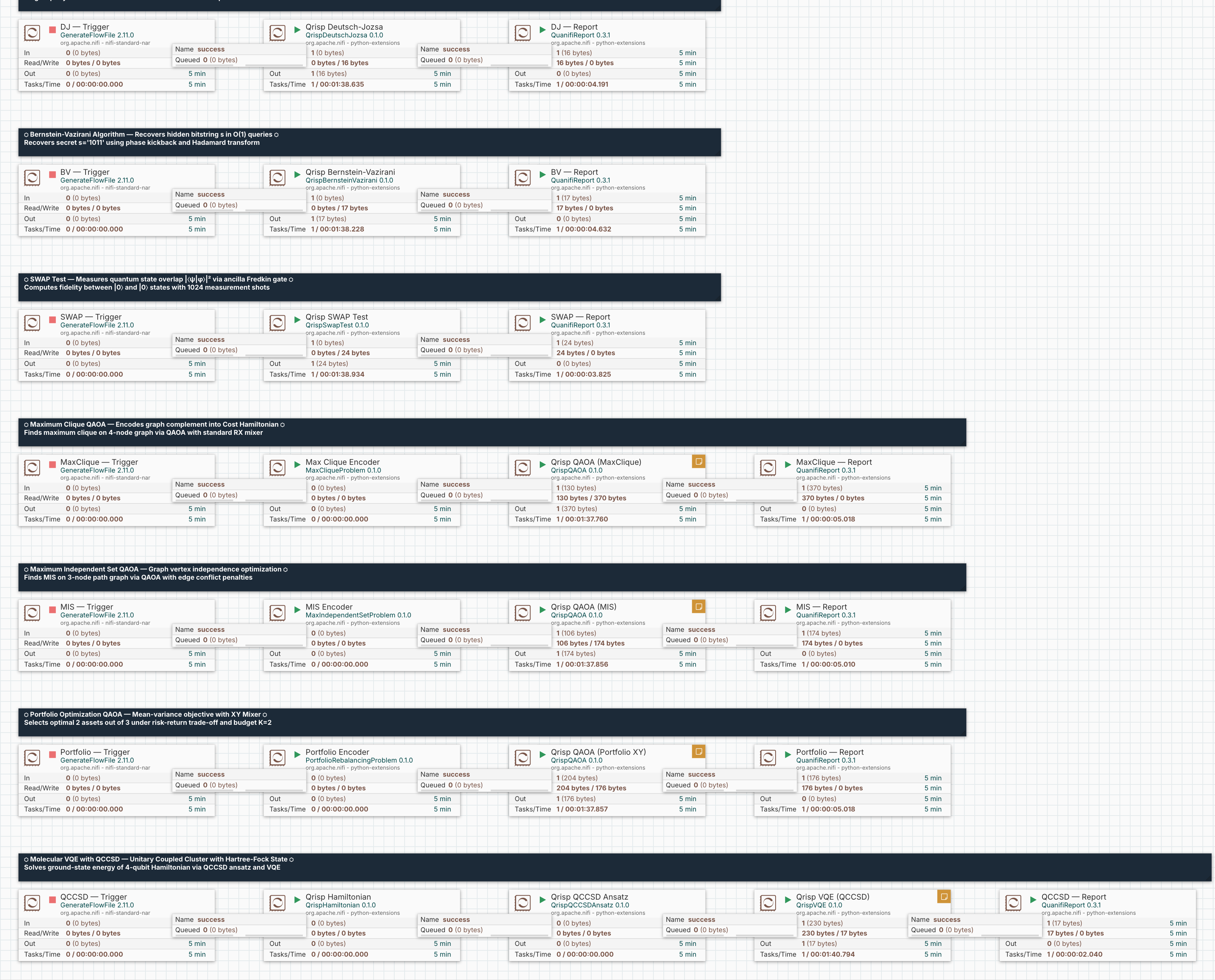
Figure 5.1: Decoupled Portfolio Rebalancing QAOA pipeline on the NiFi canvas. 🔍 Click image to enlarge in lightbox

The 6 Decoupled Stages:

1

Trigger (GenerateFlowFile)

Initiates a rebalancing assessment (e.g. daily, hourly, or market-event driven).
2

Problem Encoder (PortfolioRebalancingProblem)

Takes financial market inputs (expected returns, covariance matrix, risk aversion factor $\lambda$, budget $K$), performs the Pauli substitution, and emits a framework-neutral JSON Hamiltonian (sparse_pauli_op_json). No quantum code required for the financial analyst!
3

Variational Quantum Solver (QrispQAOA)

Consumes the Hamiltonian. Configured with Mixer Type = XY and Optimizer = COBYLA. It initializes the $K$-hot subspace, constructs the parameterized cost and mixer unitary layers $U(C, \gamma) U(M, \beta)$, and optimizes the angles in a loop. Since 0.2.0 it trains and emits the trained circuit as OpenQASM 2.0 — it no longer samples or has a Shots property.
4

A Simulator (e.g. PennylaneSimulator)

Any counts-emitting simulator can sample the trained circuit — the example canvas uses PennylaneSimulator, but any of the seven counts engines works.
5

Framework-Neutral Scorer (QuantumQAOAEvaluator)

Reads the sampled counts plus the cost Hamiltonian (carried through as hamiltonian.json) and computes every sample-dependent QAOA metric: best measurement, approximation ratio, and the rest of the qaoa.* panel.
6

Automated Reporter (QuanifiReport)

Receives the counts and the evaluator's attributes and writes the interactive audit card to reports/qrisp-qaoa-portfolio.html.

6. How to Read and Interpret the Results

Trigger the flow in NiFi, or regenerate the local example canvas and reports with:

.venv/bin/python tools/build_qaoa_examples.py --run

(the qrisp-qaoa lane covers this pipeline) and open the generated report:

open reports/qrisp-qaoa-portfolio.html

The table below is a real measured run of the qrisp-qaoa lane (demo/qaoa/lanes/qrisp-qaoa.json), Layers 2, Random Seed 11, sampled by PennylaneSimulator at 1024 shots:

Attribute	Observed Value	Financial & Quantum Interpretation
`sim.top_result`	`001`	The most frequently sampled binary vector of chosen assets — can differ from the lowest-energy one below, since it is the sampled mode, not the minimum.
`qaoa.best_measurement`	`011`	The observed bitstring with the lowest cost, from `QuantumQAOAEvaluator` — the actual portfolio recommendation.
`qaoa.mixer_type`	`XY`	Confirms the subspace-preservation mixer was applied.
`qaoa.optimal_value`	`1.83382615`	The minimized objective cost found by COBYLA (Qrisp's exact, rounded objective — see the QAOA components guide's energy-rounding note).
`qaoa.cost_function_evals`	`47`	Number of variational optimizer evaluations (this replaces the old, removed `qaoa.iterations` attribute).
`qaoa.approximation_ratio`	`1.0`	From `QuantumQAOAEvaluator`: the sampled best measurement reached the true minimum energy of this 3-asset instance.
`sim.shots`	`1024`	Statistical sampling size — now comes from the simulator stage, not the solver.

Hands-on Exercise 5.1

Tuning the Risk Aversion Factor

In portfolio management, increasing the Risk Factor ($\lambda$) forces the optimizer to avoid volatile assets, even if they have higher expected returns.

Consider 3 assets with expected returns $\mu = [0.10, 0.20, 0.15]$ and covariance diagonal (variances) $\Sigma_{ii} = [0.05, 0.08, 0.06]$.
Notice that Asset 1 (return 0.20) is the most profitable, but also the most volatile ($\Sigma_{11} = 0.08$).

Your Task:

In the NiFi canvas (https://localhost:8443/nifi), stop Portfolio Encoder.
Configure it and change the Risk Factor property from 0.5 to a high risk aversion of 5.0. Apply changes and restart the processor.
Trigger the pipeline: right-click Portfolio — Trigger and choose Run Once.
Inspect the newly appended report card in reports/qrisp-qaoa-portfolio.html.
Which 2 assets are selected now, and why did the optimal portfolio change?

👉 Click to Reveal Exercise Solution & Explanation

Solution:

With risk factor $\lambda = 5.0$, the optimizer heavily penalizes the volatility term $\lambda x^T \Sigma x$.

Selected Portfolio: 101 (Asset 0 and Asset 2).
Why: Asset 0 (variance 0.05) and Asset 2 (variance 0.06) have much lower risk than Asset 1 (variance 0.08). When risk aversion is high ($\lambda = 5.0$), the mathematical penalty of Asset 1's volatility outweighs its extra $5\%$ return!
Constraint Preservation: Notice that even though the optimal choice flipped, the measured bitstring still has exactly two 1s (101), because the XY Mixer prevents the quantum state from ever sampling illegal allocations like 111 or 100!