
Module 4: Grover's Search Algorithm
Discover how quantum amplitude amplification searches unsorted databases and inverts hash functions in $O(\sqrt{N})$ queries — achieving a provable quadratic speedup over all classical algorithms.
1. The Problem: Searching an Unsorted Database
In classical software engineering, binary search requires a sorted array ($O(\log N)$). But what if the data is completely unsorted, or you are trying to invert a one-way cryptographic hash function:
def find_preimage(target_hash: str) -> str:
    # We must find 'x' such that sha256(x) == target_hash
    ...
For an unsorted keyspace of $N = 2^n$ elements:
- Classical Brute Force: You must test items one-by-one. On average, it requires $\frac{N}{2}$ checks, and in the worst case $N$ checks ($O(N)$ linear search).
- Grover's Algorithm: Finds the unique target item with high probability in roughly $\frac{\pi}{4}\sqrt{N}$ queries ($O(\sqrt{N})$ quadratic speedup).
| Search Space ($N$) | Classical Linear Search ($N$) | Grover's Quantum Search ($\approx \frac{\pi}{4}\sqrt{N}$) | Quantum Speedup Factor |
|---|---|---|---|
| $2^4 = 16$ | $16\text{ queries}$ | $3\text{ queries}$ | $5\times$ faster |
| $2^8 = 256$ | $256\text{ queries}$ | $12\text{ queries}$ | $21\times$ faster |
| $2^{20} \approx 1,000,000$ | $1,000,000\text{ queries}$ | $785\text{ queries}$ | $1,273\times$ faster |
2. How It Works: Amplitude Amplification
Grover does not magically "look at everything at once" and return the answer. Instead, it uses a two-step cycle repeated $R$ times that gradually amplifies the target's probability amplitude while suppressing all non-targets.
The 3 Stages of Each Grover Iteration:
- Uniform Superposition: All $N$ basis states begin with identical positive amplitudes $\alpha_i = \frac{1}{\sqrt{N}}$.
- The Phase Oracle ($O$): When passed through the oracle, the marked target state $\vert\omega\rangle$ is flipped negative: $$\vert\omega\rangle \to -\vert\omega\rangle$$ All other $(N-1)$ unmarked states remain unchanged.
- The Diffusion Operator ($D$ — Inversion About the Mean): Every amplitude $\alpha_i$ is reflected across the average amplitude $\mu$: $$\alpha_i^{\text{new}} = 2\mu - \alpha_i$$ Because the target amplitude was negative, reflecting it across the mean $\mu$ causes its height to leap high above the rest, while the unmarked states sink downwards!
Unlike classical algorithms where running more iterations always gets you closer to an answer, Grover's search rotates the quantum state vector in 2D Hilbert space like the hands of a clock. The optimal iteration count is: $$R \approx \left\lfloor \frac{\pi}{4}\sqrt{N} \right\rfloor$$ If you continue past $R$, the vector rotates past the target, and the probability begins decreasing back toward zero!
3. Running Grover's Search in Quanifi
In Quanifi, Grover's search is implemented with native multi-framework support. You can construct and simulate Grover circuits with Qiskit, Cirq, or Qrisp using the exact same pipeline topology.
The Pipeline Structure:
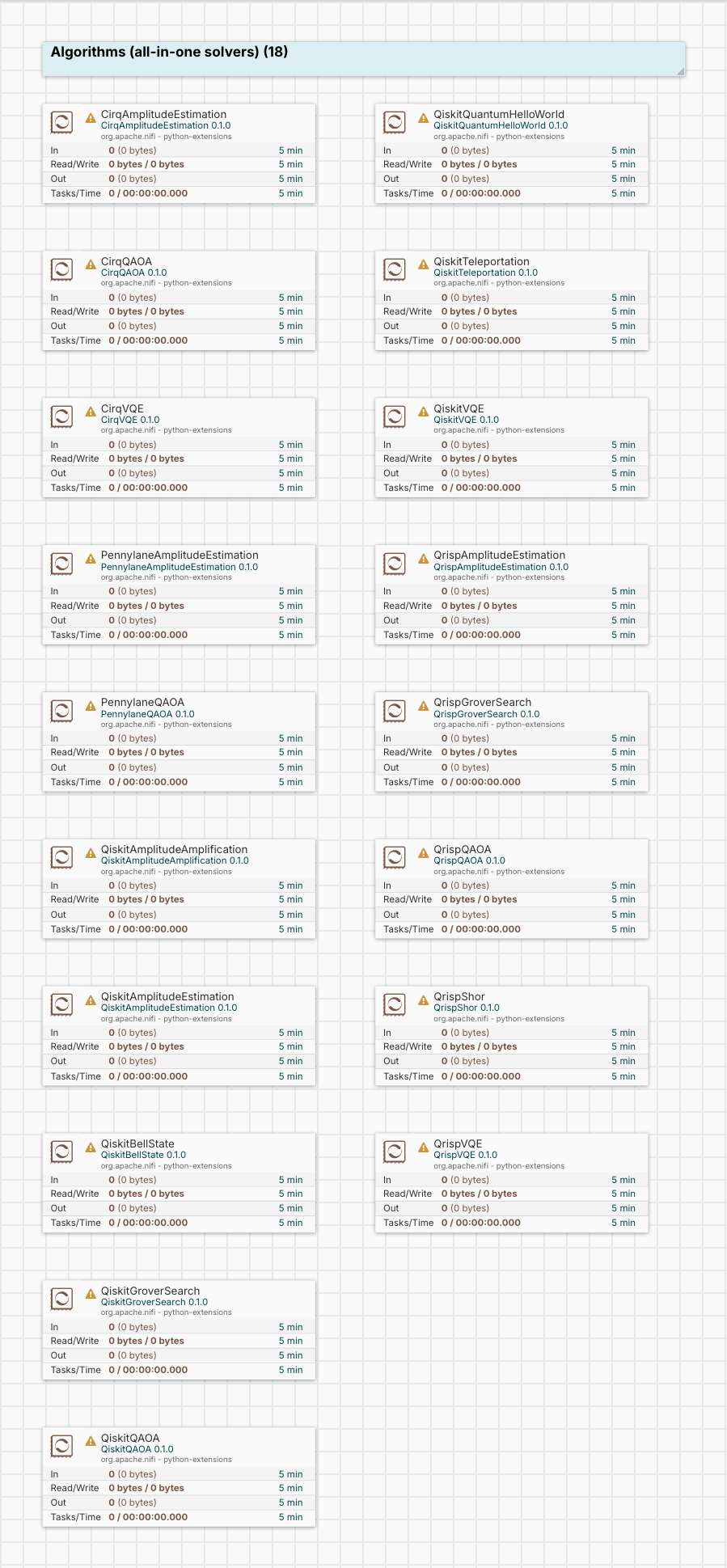
Configuring QiskitGroverSearch:
| Property | Default | Description |
|---|---|---|
| Marked State | 11 |
The binary bitstring to search for. The string length determines the number of qubits ($n$). |
| Num Iterations | 1 |
Number of oracle + diffusion cycles to apply ($R$). |
| Shots | 1024 |
Total times to sample measurement readout. |
4. Reading and Interpreting Results
When Grover finishes, the terminal QuanifiReport generates a report card showing the measurement probability distribution.
Expected Probability vs Number of Iterations:
For a 2-qubit system ($N=4$) with target 11:
- Optimal iteration count: $R = \left\lfloor \frac{\pi}{4}\sqrt{4} \right\rfloor = \left\lfloor \frac{\pi}{2} \right\rfloor = 1$ iteration.
- For $R=1$, the target probability is exactly 100% in a fault-free simulator!
- Every single one of the 1024 shots will measure
11.
For larger qubit sizes ($n \ge 3$), the probability does not hit exactly 1.0, but peaks close to $1 - \frac{1}{N}$.
Calculating Optimal Iterations and the Overcooking Effect
Suppose you are configuring a 3-qubit Grover pipeline ($n=3$) searching for the target bitstring 101 among $N = 2^3 = 8$ items.
Questions:
- Calculate the theoretical optimal number of iterations $R_{\text{opt}} \approx \left\lfloor \frac{\pi}{4}\sqrt{N} \right\rfloor$ for $N=8$.
- If you run the algorithm with only $R = 1$ iteration, will the target probability be higher or lower than at $R_{\text{opt}}$?
- If an operator mistakenly sets $R = 4$ iterations, what will happen to the measurement probability of
101?
👉 Click to Reveal Exercise Solution & Explanation
Solution:
-
Optimal Iteration Calculation:
$$R_{\text{opt}} \approx \left\lfloor \frac{\pi}{4}\sqrt{8} \right\rfloor \approx \lfloor 0.7853 \times 2.8284 \rfloor = \lfloor 2.22 \rfloor = 2\text{ iterations}$$
Applying $R = 2$ iterations maximizes the probability of measuring
101at approximately $94.5\%$! -
At $R = 1$ iteration (Under-rotated):
The state has only completed one rotation. The probability of measuring
101is approximately $78.1\%$. While significantly higher than random guess ($12.5\%$), it has not yet reached its peak. -
At $R = 4$ iterations (Overcooked / Over-rotated):
Because amplitude amplification is periodic like a sine wave $\sin^2((2R+1)\theta)$, running 4 iterations rotates the state vector past the target state! The probability of measuring
101plummets down to approximately $16.5\%$ (barely above a random guess).
Engineering Rule: In quantum pipelines, never use a "more iterations is better" heuristic. Always calculate and tune $R$ strictly based on the search space size $\sqrt{N}$.